Understanding Convolutional Neural Networks

Convolutional Neural Networks, or CNNs, have revolutionised computer vision, enabling machines to understand visual data. These deep learning models are tailored for image processing, automatically learning and extracting features. In this blog post, we’ll take a closer look into CNN concepts like weights, biases, and convolution. If you’re looking for the TLDR, check out the diagram & text below. 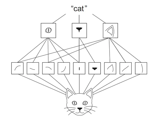Here’s how the CNN works: it starts by taking our input image (like our feline friend here) and uses convolution to auto-learn and pull out features from the image. Next, pooling steps in to distill those features into recognizable patterns—think whiskers, noses, or ears. Finally, the fully connected layer dives in, making the final call that, yup, it’s a cat. If your curiosity’s piqued and you wanna dive deeper, keep on reading!

Neurons

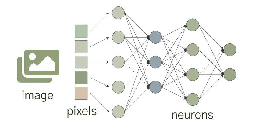
To start with, lets talk about neurons. Neurons, also sometimes referred to as nodes or units, are the fundamental operational units driving CNNs. Each neuron receives inputs, processes them using the weights and biases before generating an output. In context of an image, the inputs to a neuron could be pixel values of the image or output from previous layer’s neurons.

Weights and Biases

Weights and biases are critical components of CNNs. They are essentially learnable parameters that allow the network to adapt and improve its predictions over time. Each neuron in a CNN is associated with a weight, which determines the influence of the neuron’s input on the output. The network learns these weights through a process called backpropagation, where it adjusts them based on the errors made during training.

In addition to weights, CNNs utilise biases to introduce flexibility and control into the network. Biases act as an additional input to each neuron and help in adjusting the output. They play a crucial role in ensuring that the network can learn and generalise well, even in the presence of complex data.

Convolutions

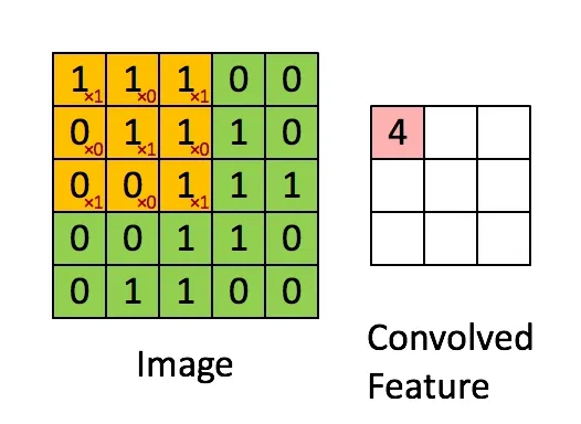
Convolution is at the heart of CNNs and is instrumental in capturing important local patterns and features from images. Convolution involves the iterative application of a filter or kernel to an input image, producing a feature map that highlights particular characteristics. The filter is a small window of values (weights) that slides over the entire input, computing dot products at each position to generate the feature map.

This convolution operation preserves spatial information, allowing the CNN to understand the spatial relationships between pixels. By preserving these relationships, CNNs can recognise objects or features in images regardless of their position. This is a key advantage over traditional neural networks that process inputs in a flattened form, losing valuable spatial information.

Activation Functions

Activation Functions play a pivotal role in shaping the output of a deep learning model, influencing its accuracy, and impacting computational efficiency. They introduce non-linearity into the network, allowing it to learn complex relationships within the data. Here are some commonly used activation functions:

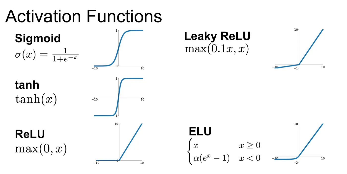
1. Sigmoid: The Sigmoid or logistic function is characterised by an ‘S’ shaped slope and is defined as:

The output of the sigmoid function ranges between 0 and 1, classifying it as a binary classification function. It's widely used in binary classification problems, logistic regression and it's excellent for implementing in the output layer for binary output models. However, it's less favoured in more complex, multi-layer networks due to two major pitfalls - vanishing gradients and lack of zero-centered output.

2. Tanh: The Hyperbolic Tangent function (Tanh) is essentially a rescaled version of the sigmoid function, with output range from -1 to 1:

The range of the tanh ensures that data is zero centered, making it slightly better than the sigmoid function for hidden layers. However, it still suffers from the problem of vanishing gradients in deep networks.

3. ReLU (Rectified Linear Units): ReLU is the most popular activation function in the field of deep learning. Mathematically, it is represented as:

The ReLU activation function introduces non-linearity to the network, setting all negative values to zero. While this allows the model to solve complex problems and maintain computational efficiency, it can also lead to the 'dying ReLU' problem, where neurons can sometimes become inactive and stop learning entirely.

4. Leaky ReLU : It’s a variation of the ReLU function that attempts to solve the dying neurons problem in ReLU and is expressed as:

It gives an extremely small linear component of x (which in this case is 0.1) for input less than 0. It remains efficient and has all the advantages of ReLU, plus it maintains some information even when x < 0.

5. Softmax : Primarily used in multi-class classification problems, softmax squashes a K-dimensional vector of arbitrary values to a K-dimensional vector of real values between 0 and 1.

6. ELU (Exponential Linear Unit): ELU is an activation function defined as:

ELU combines the benefits of ReLU and Leaky ReLU while addressing some of their limitations. It introduces non-linearity, prevents the vanishing gradient problem, and maintains computational efficiency.

Pooling or Sub-Sampling Layers

These layers are used to reduce the dimensionality of each feature map while retaining the most important information. Pooling can be of different types, such as Max, Average, or Sum. The most commonly used pooling operation is max pooling, where the maximum value within each pooling region is selected as the representative value for that region.

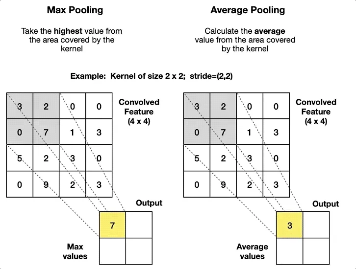
Mathematically, max pooling can be represented as:

for a given region, where F(I) represents the pooled feature map and I(x, y) represents the feature map values within the pooling region. This process helps in reducing computational complexity while preserving key features and spatial information.

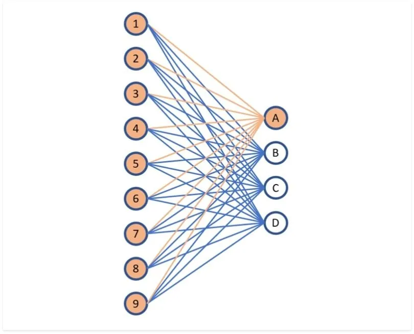
Fully Connected Layers

These layers are responsible for recognising and classifying objects in the image. Also known as dense layers, they take the information from the previous layers and make final predictions based on learned patterns and features. Each neuron in a fully connected layer is connected to every neuron in the previous layer.

Mathematically, the output value of a neuron in a fully connected layer can be calculated using the formula:

where h(x) represents the output, Σ represents summation, w represents the weights of the connections, x represents the input values from the previous layer, and b represents the bias term. The weights and biases are learned during the training process through techniques like gradient descent.

Famous Architectures

Convolutional Neural Networks (CNNs) have various architectures, each with a unique design and purpose. Let’s explore some of the well-known ones:

1. LeNet: Introduced by Yann LeCun in 1998, LeNet was primarily designed for digit recognition tasks such as ZIP code and digit recognition in bank check amounts. It is one of the earliest and simplest CNN architectures, containing only 7 layers.

2. AlexNet: Developed by Alex Krizhevsky, this network outperformed all the traditional methods in the ImageNet Large Scale Visual Recognition Challenge (ILSVRC) in 2012. AlexNet, with its eight layers, was the first to leverage the computational power of GPUs.

3. VGGNet: This architecture, developed by the Visual Graphics Group at Oxford (hence the name VGG), is famous for its simplicity. The network uses only 3x3 convolutional layers stacked on top of each other in increasing depth, reducing volume size.

4. GoogLeNet (Inception): Developed at Google, GoogLeNet introduced a novel architectural idea, the Inception Module, resulting in a deeper yet computationally cheaper model. This won the ILSVRC 2014 competition.

5. ResNet: Introduced by Microsoft, ResNet (Residual Network) introduced residual learning with “shortcut” connections to solve the vanishing gradient problem in deep architectures. With architectures as deep as 152 layers, ResNet won the 2015 ILSVRC competition.

Challenges and Limitations of CNNs

Common issues encountered during implementation

While CNNs are powerful tools for image analysis, implementing them often comes with challenges. These include overfitting, where the network performs well on the training data but poorly on unseen data; vanishing gradients, which makes it difficult for the network to learn; insufficiently diverse data leading to biased model; and computational expense in training large models.

Limitations of CNNs

Despite their success, CNNs also have limitations. They require large amounts of labeled data for training, which can often be time-consuming and costly to obtain. More so, they lack interpretability, i.e., it’s difficult to understand why a CNN made a certain prediction, limiting their usage in scenarios where interpretability is necessary, such as medical diagnosis. Furthermore, CNNs assume that all inputs (like images) are grid-like, which restricts their applicability to other types of data. Lastly, they are sensitive to the size and orientation of objects in the input images, and may fail with objects of unusual sizes or orientations.

Going Forward: Applications and Future Developments

Convolutional Neural Networks find applications in diverse fields, thanks to their ability to analyse and interpret visual data. Some notable applications include:

• Image and Video Processing: CNNs are used for video interpretation, image recognition, and classification tasks.

• Autonomous Vehicles: Self-driving cars heavily rely on CNNs to detect objects and people on the road, enabling safe navigation.

• Healthcare: CNNs aid in the detection of diseases in medical imaging, assisting doctors in making accurate diagnoses.

• Face Recognition: CNNs are increasingly utilised for recognising faces and facial expressions, playing a crucial role in biometric security systems.
  
  

I hope you have found this blog helpful !