
Table of contents
- 1. Executive Summary
- 2. Data Preprocessing
- 3. Methodology / Methods of Data Mining
- 4. Modelling
- 5. Experiment Analysis
- 6. Model Comparison
- 7. Model Assessment
- 8. Model Deployment
- 9. Conclusion
- 10. Appendix
- 11. Reference List
1. Executive Summary
A comprehensive analysis was conducted using five distinct models within the context of a car auction business. The primary objective was to predict whether a vehicle is a “Bad Buy.” The project commenced with rigorous Data Preprocessing, involving the meticulous handling of missing values, outliers, and data noise within a car sale dataset. We also selected and justified relevant features, ensuring a robust foundation for predictive modelling in the specific context of the auction market.
Subsequently, we systematically employed methods like Random Forest and Neural Networks in the Methodology and Methods of Data Mining phase. Clear explanations and justifications underpinned our method selection, ensuring that our analysis was finely tailored to the unique intricacies of the car auction business. Through thoughtful model selection and parameter tuning in the Modeling phase, we optimised our models for the task of accurately predicting “Bad Buy” vehicles. The Experiment Analysis offered detailed insights through visualisations, facilitating data-driven decision-making within the car auction sector. Finally, our project’s Model Assessment highlighted the robustness of the champion model, underscoring its reliability in making predictions vital to the car auction business. In conclusion, our project provided valuable insights for more informed decision-making in the car auction business and offered suggestions for future research and improvements in this unique sector.
2. Data Preprocessing
Data preprocessing for our dataset encompassed essential steps involving data exploration, imputation, and variable selection nodes. The Variable Selection node played a pivotal role in determining which input variables were accepted and rejected. Meanwhile, the Imputation node was employed to address missing data, and the Data Exploration node facilitated feature selection. No transformations techniques were applied to any of the input data besides handling missing inputs.
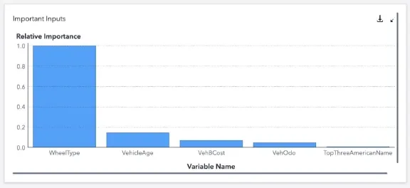
Using the data exploration node, a comprehensive analysis of the chosen dataset was conducted, offering summary statistics and insightful plots for each variable. This process unveiled the key input variable for our target variable, isBadBuy with WheelType emerging as the most influential, followed by VehicleAge.
Additionally, an imbalance in the distribution of our target variable was observed, with over 87% of isBadBuy values being 0, signifying ‘not a bad buy,’ which could potentially impact the model’s learning.
The data exploration node also allowed us to visualize the relationship between the target variable and the input variables. For instance, the correlation between isBadBuy and VehicleAge became apparent, highlighting that older vehicles are more likely to be classified as a bad buy. Consequently, incorporating VehicleAge as an input variable was deemed advantageous for the model training process.

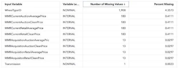
To ensure the proper handling of missing values, the imputation node was utilized. Default parameters were employed, indicating that missing nominal variables were replaced using the mode, while missing interval variables were substituted with the mean. A table was generated to display the extent of missing values in our dataset, revealing the percentage of missing data for each variable.
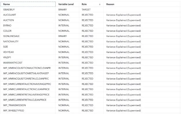
The variable selection node employed a combination of unsupervised and supervised methods for reducing the number of input variables. Default parameters, specifically the Fast Supervised Selection method, were applied. The outcome of this process is reflected in a table showcasing the target variable and the list of rejected variables.
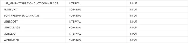
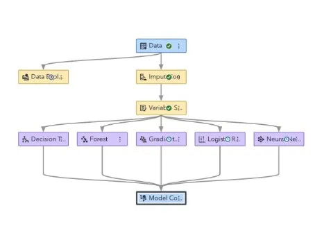
Finally, the input variables that were retained for the decision tree model are illustrated in the figure below, emphasizing that the joint use of the variable selection node with default parameters and the data exploration node justified the selection of these specific input variables.
In summary, we improved the prediction of auction sales being a bad buy by selectively choosing input variables via the Variable Selection node. Missing data was handled using the Imputation node, ensuring clean data for training. The Data Exploration node justified the inclusion of crucial variables like VehicleAge to enhance predictive performance. Given the binary output, no normalization or transformation techniques were required.
3. Methodology / Methods of Data Mining
To develop the model we utilised the SAS VIYA Model Builder, this is a powerful tool which is capable of analysing a number of different models almost simultaneously, by simplifying the model development process in this way we were able to more efficiently explore a number of models and assess the best output based on a number of metrics. In order to utilise a number of different modelling methods we elected to explore: Logistic Regression, Decision Tree, Random Forest, Gradient Boosting and Neural Network models. Analysing a number of models in this way allowed us to determine the best model type for the dataset prior to commencing hyperparameter tuning to optimise performance.
The data we are using in this model was missing a number of variables which needed to be imputed as described earlier in this report, furthermore given the nature of this prediction as a binary classification problem it can be deduced that the random probability of the model would be 50% as such each model must perform significantly over 50% accuracy to be considered effective.(Naik & Purohit, 2017) Many of the variables are related to a vehicle’s price which may skew the model due to the variability in vehicle pricing. As a result it may be necessary to tune parameters appropriately to account for these outlying data points.
The pipeline illustrated in the figure above allowed us to explore a number of models simultaneously, all of the explored models performed exceptionally well “out-of-the-box” with classification accuracies of greater than 85% on the binary classification task, we discovered that the Random Forest classifier offered the best untuned final results this model leverages a number of decision trees to arrive at a prediction as a result it utilises many of the strengths of a Decision Tree Classifier while increasing the overall power of the model as expected of an
ensemble learner, for this reason it is understandable that the model performed with a high level
of accuracy. Random Forest Classifiers have the additional benefit of being interpretable systems meaning we do not need to deal with the “Black-Box” problem of AI which is an additional benefit when proposing this system to stakeholders. (Breiman, 2001)
Once we determined that the Random Forest Classifier was our preferred model for further development we began to experiment with varying settings in this node within SAS VIYA Model Builder to determine if there would be a significant performance boost without significant resource penalty, the results of this exploration will be more deeply exploited in the Results Analysis section of the report. In the development of these models we explored a number of model architectures and imputation methods to ensure we were producing the most appropriate final model capable of performing with the highest overarching accuracy.
4. Modelling
1. Algorithm Selection
The algorithm we use to create our model is very important as each have their own positives and negatives for different datasets. Below we will discuss each algorithm we have experimented with to find the best results.
Decision trees are a broader family of tree-based algorithms. They function by partitioning the dataset into subsets based on feature values, essentially breaking down a complex decision-making process into a combination of simpler decisions, represented in a tree-like mode. Each node of the tree represents a decision based on the value of one input feature, leading to branches and eventually terminating at leaves which represent the final decision or prediction. In terms of our CarData set, our input variables act as the branches which lead to the IsBadBuy variable representing 0 or 1. A major strength of decision trees is their interpretability as it can be easily understood. The algorithm can handle both numerical and categorical data, and while preprocessing like normalization isn’t mandatory, handling missing values and reducing dimensionality can improve performance. However, it’s essential to be cautious of overfitting, where the tree becomes too complex and tailored to the training data, limiting its ability to generalize well to new data. Factors like data size and the complexity of relationships may hinder the decision tree from being the optimal choice.
Neural networks are a subset of machine learning algorithms that consist of interconnected nodes or “neurons” organized in layers, inspired by the human brain’s architecture. These layers capture intricate patterns and relationships in data through a process of weighted inputs and activations. Particularly for our CarData set, this algorithm is able to identify the relationship between the input variables like the VehOdo and size.They thrive on large datasets and can handle diverse data types, including numerical, categorical, text, and even images. One of the significant advantages of neural networks is their ability to model complex, non-linear relationships without manual feature engineering, making them particularly powerful for intricate datasets. Unfortunately, due to neural networks adaptability and complexity, they are notoriously “black-box” models, making their predictions difficult to interpret. With our dataset, they will be difficult to explain why the car is considered a bad buy for consumers. They can also be computationally expensive to train, especially deep neural networks with many layers. Overfitting can be an issue if not enough data is available or if the model is overly complex, necessitating techniques like dropout or regularization to mitigate. Proper network design and hyperparameter tuning are essential to harness their full potential effectively, but may be too complex for the CarData set we are classifying
Gradient Boosting is a ensemble machine learning algorithm that builds a series of weak models, like decision trees, in a sequential manner. Different to other ensemble methods that build trees independently, Gradient Boosting improves on errors by adding trees that correct the mistakes of the previous ones, essentially optimising a loss function by gradient descent, adding one tree at a time to minimize the error. One of the positives of Gradient Boosting is its high predictive accuracy as it uses multiple methods and tends to be more complicated. Additionally,
it can handle missing data, and offers insights into feature importance, aiding in understanding the driving factors behind predictions. However, on the downside, Gradient Boosting can be computationally intensive and time-consuming, especially with large datasets. It’s also more prone to overfitting, especially with noisy data, compared to Random Forest. Lastly, while it provides excellent predictive power, its ensemble nature can make it less interpretable than simpler models like a single decision tree.
Logistic Regression is a statistical algorithm which predicts the probability that a given instance belongs to a particular category. In terms of our CarData set, we use input variables such as size, VehicleAge, VehOdo, WheelType and more to identify the target variable of IsBadBuy (with values 0 and 1 representing no and yes). The model estimates this probability by fitting data to a logistic curve (S-curve). It takes in any number of input variables, which can be either numerical or categorical, and predicts a binary outcome – 0 or 1. Our Cardata set is quite suitable for this kind of analysis as each instance in the dataset has a set of features and a binary outcome label. Proper feature engineering and preprocessing, such as handling missing values, encoding categorical variables, and scaling numerical variables, are crucial for the effective application of logistic regression. Its strength lies in its ability to provide a probabilistic interpretation for predictions and its efficiency in dealing with datasets that have linear decision boundaries. Furthermore, when regularized, it tends to be resistant to overfitting, enhancing its generalization capabilities. However, it does come with limitations. The model assumes a linear relationship between the features and the log-odds of the dependent variable, making it less effective for data with complex, non-linear decision boundaries. Additionally, when handling high-dimensional datasets, feature selection becomes pivotal, as it’s not inherently suited for such data. Proper preprocessing is essential since it’s sensitive to feature scaling, and its performance can be compromised if this step is overlooked.
Random Forest is an ensemble learning algorithm that builds upon the concept of decision trees. Instead of relying on a single decision tree, Random Forest constructs multiple trees during training and combines their outputs for more robust and accurate predictions. They build on this idea by including the random aspect, by bootstrapping the training data for each tree and by randomly selecting a subset of features for every split in each tree to limit the affect of overfitting. The model thrives on datasets with mixed data types (both numerical and categorical) and is adept at handling large datasets with complex, non-linear relationships. Some positives of Random Forest include its high accuracy, ability to rank feature importance, and its robustness against overfitting due to the ensemble approach. However, negatives encompass its computational intensity when building a large number of trees, potential lack of understanding of decisions and the possibility of model bias if classes in the dataset are imbalanced. For our CarData, random forest bring the best of the simplicity of decision trees, whilst dealing with the limitations of a low powdered model.
2. Model Tuning
Model tuning refers to the process of adjusting the parameters of a machine learning algorithm to optimize its performance. Through this iterative procedure, practitioners aim to enhance the model’s accuracy and generalization capabilities, ensuring it performs well on unseen data. SAS offer many tuning options for all of their model. A better understanding will allow us to fine tune our model for our dataset. After various trial and error, we adjusted these settings to gain the best results for each model
Decision trees
- Grow Criterion - This relates to the metric or measure used to determine the best split at each node. This will change with the target variable, for example we use the Gini option as it is mainly used for binary classification problems. It measures the impurities of the dataset and accounts for them.
- Maximum Number of Branches - This sets an upper limit on the number of branches or splits a node can have. This is mainly only changed if computational time is a concern.
- Maximum Depth - It restricts how deep the tree can grow. This is essential to prevent overfitting of deeper trees. If validation accuracy is lower than training accuracy, this may need to be reduced.
- Minimum Leaf Size - Ensures that a leaf (final node) has at least a minimum number of observations. This will prevent overfitting if we have a smaller dataset or many outliers.
- Handling Missing Values - Specifies how the decision tree should handle instances with missing values. As we have a low percentage of missing values ( with less than 0.5% for most values and less than 5% of our most missing value row, being WheelTypeID ), we can use them in search.
- Minimum Missing Use in Search - Defines a threshold for the minimum number of missing values needed to consider a surrogate split. As we do not have any surrogate rules (due to little missing values), this option does not matter.
- Number of Interval Bins - Involves discretizing continuous variables into a specified number of bins. For more complex distribution, we use more bins which is why we chose 50 interval bins.
- Interval Bin Method - Determines the methodology for binning. As we have complex data, we use Quantile Binning so each value is handled itself and not uniform.
- Surrogate Rules - These are backup rules or splits that are used when a primary split’s conditions can’t be met due to missing values. As we have a low percentage of missing values, we do not need to make surrogate rules and set it to 0.
- Using Input Once - Ensures that a particular input or feature is used only once in the decision-making process of the tree. This is mainly enabled if you have high correlation of values, which is not the case for our dataset.
- Perform Clustering Based Split Search - This is an advanced feature where the algorithm might look for splits based on clustering patterns within the data.
- Pruning Options - This pertains to the initial subsets of data used in the pruning process. If suspect overfitting, you can increase the number of seeds to simplify the model.
- Binary Classification Cutoff - For binary classification tasks, this threshold determines when to classify an instance as one class over the other based on predicted probabilities. You can adjust this if false positives are being more common.
Neural Networks
- Input Standardization - If the features in your dataset have vastly different scales or units, standardization becomes vital. We use the midrange satndardisation to limit the affect of outliers
- Number of Hidden Layers - Influences the network’s capacity to capture complex patterns. More layers can model more complexity but risk overfitting. Due to this we limit the hidden layers to 1.
- Use Same Number of Neurons in Hidden Layers - For simplicity, one might choose the same neuron count across layers. Different counts can capture patterns at varying scales.
- Number of Neurons Per Hidden Layer - A critical parameter affecting capacity and computation. More neurons increase capacity but can also risk overfitting. We use a generic number of 50.
- Hidden Layer Activation Function - Choosing the correct function allows networks to learn intricate patterns as it creates non-linearity. This is why we choose the tanh option, after experimenting with each function.
- Interval Target Standardization - Relates to the type of distribution that best describes the target variable. As the target variable is a binary problem, each is option is not very applicable but normal is the best.
- Interval Target Activation Function - Defines the function applied to the output. We choose identity for this which means the output of the neruon is the same as the input for linear function.
- Optimization Method - To ensure quicker convergence and better generalisation. We choose automatic to allow for the software to choose the best option for us
- Number of Tries - How many times the model should be initialized and trained. We set this to 1 to restrict overfitting the model
- Maximum Iterations - Upper limit on the number of epochs. We set this to a generic 300.
- Maximum Time - Upper limit on training time.
- Random Seed - Ensures reproducibility by setting a seed for random number generation. The number you choose is not really important, as it is random.
- Layer 1 & Layer 2 Weight Decay - These settings control the networks capacity. We set these to 0 and 0.1 to avoid overfitting
- Input Layer Dropout Ratio & Hidden Layer Dropout Ratio - Dropout is a technique to prevent overfitting by randomly ignoring a fraction of neurons during training.
- Stagnation - Stop training if the model isn’t improving after a set number of epochs. We set this number to 5.
- Validation Error Goal - Stop training once the validation error is below a certain threshold. We set this to 0 as we want to limit validation errors.
Gradient boosting
- Number of Trees - Refers to the number of sequential trees being modeled. This is important as more trees can capture more intricate patterns, but at the risk of overfitting. We use a generic number of 100, the same as our other models to balance accuracy.
- Learning Rate - Dictates the step size at each iteration while moving towards a minimum of the loss function. We use 0.1 as a smaller learning rate makes the optimization more robust, but requires more trees.
- Subsample Rate - Fraction of the training data used for learning each tree. We use 0.5 as a value less than 1 can lead to regularization and better generalization.
- Layer 1 & 2 Regularization - L1 and L2 regularization terms on weights. Adds bias to prevent overfitting. We start with 0 for L1 and have 1 for L2 to add some penalty and prevent potential overfitting.
- Interval Target Distribution - Defines the distribution of the target variable. We choose normal to account for the error distribution of the residuals.
- Seed - The initial value for the random number generator. We set this to the same random number to be used for all models, 12 345.
- Maximum Number of Branches & Depth - Controls the size and complexity of trees as too many branches or too much depth can overfit the data. For this reason, we set our value low to 2.
- Minimum Leaf Size - The smallest number of samples required to form a leaf. This helps in regularizing the tree and preventing very specific splits. We set this to 5 as it might help in avoiding rare but specific scenarios.
- Missing Values & Minimum Missing Use in Search - Defines how missing values are treated. As we have a low percentage of missing values, we can use these in the search.
- Number of Interval Bins & Interval Bin Method - How continuous features are binned. This affects the splits in the tree, so we choose a quantile bin method with a generic 50 bins due to the size of the data and the irregularity of the ranges of each value.
- Use Default Number of Inputs to Consider per Split - Decides how many features are evaluated for splitting. We enable this as it can speed up training and add regularization.
- Class Target Metric - The metric used to measure classification quality. As our dataset is for binary classification problem, log loss is used as it considers the probability estimates.
- Early Stopping Method & Stagnation - Determines when to stop adding trees. We use the stagnation option so if performance on a validation set doesn’t improve for a set number of trees (5), then training can stop early, saving time and preventing overfitting.
Logistic regression
- Binary Target Link Function - Determines the link between the linear combination of predictors and the predicted probability. We choose logit as it models the log-odds of the probability of the event.
- Nominal Target Link Function: For multinomial logistic regression where target has >2 levels. We use generalised logit as our reponse categories are not ordered.
- Class Input Order - Determines how classes are ordered, which might influence reference category and interpretation. They dictate how predictor variables are added/removed. This is very specific for each dataset so we use the generic formatted option.
- Selection Method - Dictates how predictor variables are added/removed. We use stepwise manner as it moves step by step to solve a problem. It combines both forward selection and backward elimintaion methods.
- Effect Selection Criterion - Determines the statistical criteria based on which effects (predictors) are selected during model building. Aim for model parsimony and the nature of predictors. We use the Schwarz Bayesian Criterion (SBC BIC) among a finite set of models as it is an extension of the likelihood principle. It helps the model achieve a good balance between fit and simplicity. When the sample size is large, it is less likely to overfit due to the penalty factor.
- Selection-Process Stopping Criterion - Defines when to stop adding/removing predictors. To gain the balance between accuracy and complexity, we use the Schwarz Bayesian Criterion (SBC BIC) as it can look at liklihood to prevent overfitting by generalising better to unseen data.
- Model Selection Criterion - Uses statistics to compare and evaluate models to find the best. We use the Schwarz Bayesian Criterion (SBC BIC) as it rewards the models that fit the data well, but penalise too many parameters, limiting overfitting. This will handle a range of models with varying complexity.
- Maximum Number of Effects - Limits the number of predictor variables in the model. This will avoid lengthy model building processes and avoid overfitting, especially with small datasets. This is why we set our maximum to 0.
- Maximum Number of Steps - Restricts the number of steps in stepwise selection. To avoid exhaustive model-building processes and limit the computational power needed for the model.
- Hierarchy - Handles higher-order terms to focus on for model interpretability and to avoid misleading findings. As we do not have any stronger values, we can set this to none.
- Optimization Technique - We use Newton-Raphson with ridging as it is an iterative method to estimate parameters, ridging prevents convergence issues. This stablises estimations, ensuring model convergence.
Random forest
- Number of Trees - This determines how many individual decision trees will be built within the forest. More trees usually provide better generalization but at the cost of increased computation. It helps reduce the variance of the model. We choose a generic number of 100 trees after experimenting with lower and higher values.
- Class Voting Method - How each tree’s prediction is accounted for in the final decision. We choose probability as it averages out the probablities and can be more nuanced
- Class Target Criterion - The metric used to evaluate the quality of a split in classification tasks. We choose gini as the best option as it can handle binary classification the best.
- Interval Target Criterion - The metric for evaluating splits in regression tasks. This can affect the tree depth and structure. We choose variance as it makes each node as homogenous as possible
- Maximum Number of Branches - Can be used to simplify trees or handle categorical variables with many levels. We choose a low number for this to simplify and control overfitting.
- Maximum Depth - Controls overfitting; a shallower tree may generalize better but capture fewer nuances in the data. We set this to a middle number of 20 to capture the intricacies in the data, but limit overfitting
- Leaf Size Specification and Minimum Leaf Size - Prevents the tree from making splits that are too specific (and possibly overfitting). We set this to a count of 5 as a generic term after experimentation into higher and lower numbers.
- Handling Missing Values & Minimum Missing Use in Search - Determines how the algorithm should handle and split on features with missing data. As we have a low percentage of missing values ( with less than 0.5% for most values and less than 5% of our most missing value row, being WheelTypeID ), we can use them in search.
- Number of Interval Bins & Interval Bin Method - Methods to handle continuous variables by binning them.Affects the granularity of splits on continuous features. We want each value to be handled itself as input values ranges differ, so we choose quantilte.
- Inbag Sample Proportion - Proportion of training data sampled (with replacement) for training each individual tree. Influences diversity among trees; lower values increase diversity but may decrease individual tree accuracy. We choose a 60% training split to give the model enough data for accurate training, but enough testing data to recognise if the model is correctly classifying.
- Number of Inputs to Consider per Split & Number with Loh’s Method - How many features the algorithm should consider when making a split. This controls diversity and computational complexity. Considering fewer features can make forests more diverse but individual trees less optimal. We select 0 as it sets a default behaviour.
- Seed - Sets the initial state for random processes to ensure reproducibility. Different seeds can result in different forests, but we set a fixed seed random number produced every run.
5. Experiment Analysis
5.1 Experiment Setup (Final preprocessed dataset used, evaluation metrics used, describe briefly pipeline.)
Due to the change of datasets, we started our investigation with an exploratory data analysis (EDA),Identifying and removing features that had no impact on our models’ prediction value. Potential features to eliminate could then be identified by analysing the distribution, variance, and correlations between the variables. This was further proven by our pipeline’s Variable Selection node, ensuring that our initial choices were further refined as the Variable Selection node also eliminated them based on their limited predictive significance.
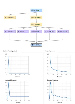
The final preprocessed dataset, which was the result of these selection and validation efforts, was then fed into a series of machine learning models. Our pipeline, as shown above, follows a logical progression of steps, starting with the ‘Data Exploration’ node. This node was utilised to understand the data distribution, missing values, and outliers. Following this, the ‘Imputation’ node addressed missing data, ensuring the models received a complete dataset.
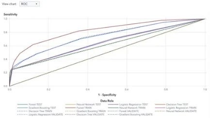
After imputation, the ‘Variable Selection’ node was utilised as it rejected inefficient variables with little potential impact to the models accuracy. The models: Decision Trees, Forest, Gradient Boosting, Logistic Regression, and Neural Networks were then trained using the dataset from this node. These models were selected because to their efficacy in binary classification problems, each of which provides a unique method for differentiating between the two groups. ROC (Receiver Operating Characteristic) curve was used as our evaluation metric due to its ability to effectively measure the performance of binary classifiers, specifically the true positive rate versus its false positive rate. A common challenge all the team members faced during this experiment was with the SAS server. On several occasions, there were issues with data not loading properly. Additionally, the project pipeline that was saves on the exchange and on the personal accounts were inadvertently deleted due to server hiccups.
6. Model Comparison
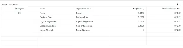
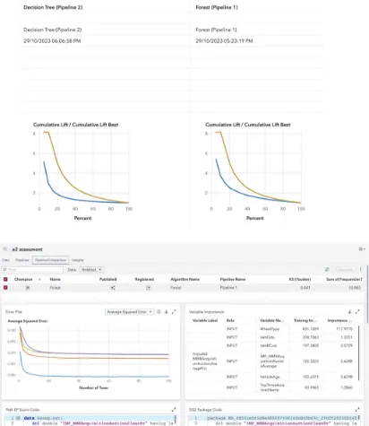
The five models that were used and then compared against each other were Decision Tree, Forest, Gradient Boosting, Logistic Regression and Neural Network. These models were all trained on the default parameters and the champion model was selected from the results which can be seen in the figure below. As we can see the random forest has one of the lowest misclassification rates meaning the overall accuracy was a lot higher.
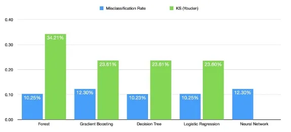
It also has the best ROC curve represented by the KS Youden which calculates the distance of the curve from the baseline model, with random forest having the highest distance. This can be seen from the chart below where the baseline model would be just a diagonal line with a slope of one.
A high KS (Youden) score is important as it shows that the model is distinguishing between classes a lot better. Subsequently, this is also evident by the AUC (area under curve) which would also be the largest for the Forest Algorithm as its KS (Youden) is higher. As can be seen below, the Model Comparison node chose the Forest Algorithm as the champion.
Finally, another reason which outlines the robustness of the random forest is its high cumulative lift which can be seen in the figure below. Cumulative lift, as depicted in the figure below, illustrates the Random Forest’s robustness in improving predictive performance over a baseline model or a random guess. This measure is essential because it demonstrates how much better the model is at identifying positive cases compared to a random selection or a basic model. The Forest Algorithm is 3.675 times better in this case.
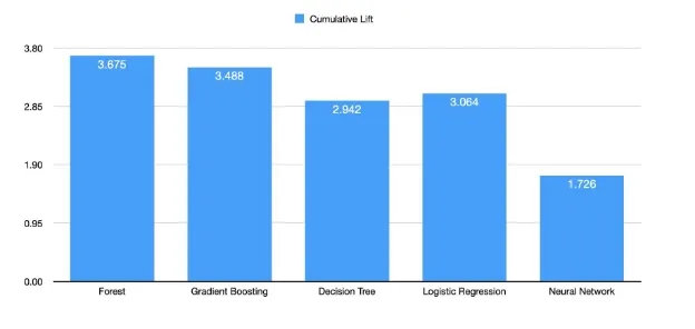
The combination of a high cumulative lift, high KS (Youden), and low misclassification rate suggests that the Random Forest model is robust and valuable for ranking and identifying positive cases, outperforming random or basic approaches. It’s important to note that these metrics indicate the model’s effectiveness in binary classification tasks and its ability to distinguish between classes, making it a strong choice for such tasks.
7. Model Assessment
7.1 Best Model - Random Forest Classifier
The best model for our chosen dataset turned out to be the Random Forest Model. As previously mentioned, the Random Forest Model Is a versatile machine learning algorithm that has gained widespread acclaim for its robustness and excellent performance in various applications. In this section, we’ll delve into what Random Forest classifiers are, why they often outperform decision trees, logistic regression, gradient boosting, and neural networks in specific scenarios, and why they are considered a robust model.
A Random Forest classifier is an ensemble learning method designed to make predictions by combining multiple decision trees. They work by creating a collection of individual decision trees, each trained on a subset of the training data.
Randomness is then introduced in two key ways: through the selection of a random subset of the training data for each tree (known as bootstrapping) and by considering a random subset of features at each split in the decision tree.
When making predictions, each tree “votes” for a class in a classification problem or provides a numerical output in a regression problem. The final prediction is determined by either taking a majority vote (for classification) or averaging the predictions (for regression).
Random Forest classifiers tend to outperform several other machine learning algorithms, such as decision trees, logistic regression, gradient boosting, and neural networks, in specific scenarios for several key reasons:
Overfitting Reduction:
Random Forests excel at mitigating overfitting, a common challenge in machine learning. By training multiple decision trees on different subsets of data, they capture different aspects of the data’s complexity, reducing variance and improving generalisation. In contrast, a single decision tree can easily overfit the data.
Robustness to Outliers and Noisy Data:
Random Forests are robust to outliers and noisy data. Since they aggregate the results of multiple trees, the impact of outliers on the overall model is minimised. Decision trees and logistic regression can be sensitive to outliers, making Random Forest a more reliable choice in such cases.
Handling Non-Linear Relationships:
Random Forests can efficiently capture non-linear relationships in the data. Decision trees may struggle with this, and while gradient boosting can handle non-linearity, it is more complex and can be prone to overfitting.
Feature Importance:
Random Forests provide feature importance scores, which can be very informative for feature selection and data analysis. This is not a feature of traditional logistic regression, and while gradient boosting and neural networks can provide feature importance, it’s usually less straightforward.
Reduced Bias:
In the case of imbalanced datasets, Random Forests are less biased compared to a single decision tree, which might favor the majority class. Gradient boosting can also mitigate this issue, but it requires careful tuning.
Handling Missing Data:
Random Forests can handle missing data gracefully. They can provide reasonable predictions even when some features have missing values, making them versatile in real-world datasets. Decision trees can be sensitive to missing data, and imputing data for logistic regression, gradient boosting, or neural networks can be challenging.
Parallelization:
Random Forests can be easily parallelized, taking advantage of multi-core processors and distributed computing environments. This makes them computationally efficient, while training deep neural networks can be time-consuming and resource-intensive.
Another advantage of RF models is that they tend to be more interpretable than deep neural networks, as they provide feature importance scores and allow for an intuitive understanding of model decisions.
Essentially Random Forest classifiers offer a robust and versatile machine learning approach that excels in various scenarios. Their ability to reduce overfitting, handle outliers and noisy data, and capture complex relationships in the data, among other advantages, makes them a reliable choice for various machine learning tasks. While Random Forests may not always outperform other models, they are often a strong contender and are particularly appealing when interpretability and robustness are crucial.
8. Model Deployment
8.1 Model Deployment Process in SAS Model Manager
To make sure the models are correctly integrated, tested, and monitored, there are multiple steps in the model deployment process in SAS Model Manager and SAS build models. Here are the steps we took to achieve this:
- Model Registration:
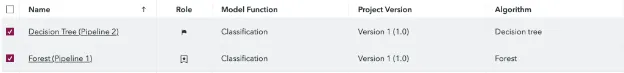
- The Champion Model (Random Forest) and the Challenger Model (Decision Tree) were registered in SAS Model Manager (as shown in the appendix).
- Registration of the models which involved uploading the model files, defining input and output variables, as well as specifying other model properties.
- Model Deployment:
- After registration, both models were deployed with their respective names.
- The reason we deploy the models is to make them accessible for scoring and ensures that they are properly integrated with the required dataset and execution environments.
- Champion-Challenger Testing:
- SAS Model Manager supports Champion-Challenger testing, which allows for two or more models to be tested against each other to compare performance.
- The Champion Model (Random Forest) and Challenger Model (Decision Tree) were deployed to evaluate their performance on the same dataset
- Scoring and Test Result Output:
- The models were used to score new data, and the results were output for analysis.
- Scoring involves applying the model to new data to generate predictions or classifications.
- Performance Evaluation and Comparison:
- The performance of the models was evaluated and compared based on the test results.
- Graphs and other tools in SAS Model Manager were used to visualise and interpret the results.
- Selection of Best Model:
- Based on the performance evaluation, the Random Forest model (Champion) was determined to be the best performing model (as shown in the appendix).
9. Conclusion
From this project, we created a successful mode using SAS Viyal for classifying CarData data set with target variable of “IsBadBuy” with low misclassification rates, demonstrationg superiority through the KS (Youden) score and indicating a robust predictive performance 3.675 times more effective than a random or basic model.
We were able to create this model after testing algorithms Decision Tree, Forest, Gradient Boosting, Logistic Regression, and Neural Network. Each was trained on default parameters for fair comparison. The Random Forest model, an ensemble of decision trees, showcased outstanding performance on multiple fronts. This was seen with the model’s advantages in handling outliers, capturing non-linear relationships, and its efficiency with missing data were evident in our results. The added benefit of feature importance scores further assisted in understanding the driving factors behind its predictions.
We were also able to learn a lot about the CarData data set with variables such as WheelType and VehicleAge identified as pivotal for predicting ‘isBadBuy’. Notably, a major portion (87%) of the dataset labeled cars as favorable purchases. This skewness could have introduced challenges for model learning, but it was evident from data visualization that older vehicles were more prone to being categorized as ‘bad buys’.
In conclusion, our experiment with the car dataset led to the conclusion that the Random Forest Classifier, given its robustness and accuracy, is an optimal choice for predicting ‘isBadBuy’. Its exceptional results not only validate our modeling approach but also highlight its potential applicability for similar classification tasks in the future.
10. Appendix


11. Reference List
All-Tanvir, A., Ali Khandokar, I., Muzahidul Islam, A. K. M., Islam, S., & Shatabda, S. (2023). A gradient boosting classifier for purchase intention prediction of Online Shoppers. Heliyon, 9(4). https://doi.org/10.1016/j.heliyon.2023.e15163
Breiman, L. (2001). Machine Learning, 45(1), 5–32. https://doi.org/10.1023/a:1010933404324
Fraj, M. B. (2017, December 24). In depth: Parameter tuning for gradient boosting. Medium. https://medium.com/all-things-ai/in-depth-parameter-tuning-for-gradient-boosting-3363992e9bae
Jain, A. (2022, June 15). Complete machine learning guide to parameter tuning in gradient boosting (GBM) in Python. Analytics Vidhya.https://www.analyticsvidhya.com/blog/2016/02/complete-guide-parameter-tuning-gradient-boosting-gbm -python
Kelkar, K. M., & Bakal, J. W. (2020). Hyper parameter tuning of random forest algorithm for Affective Learning System. 2020 Third International Conference on Smart Systems and Inventive Technology (ICSSIT). https://doi.org/10.1109/icssit48917.2020.9214213
Mithrakumar, M. (2019, November 12). How to tune a decision tree?. Medium. https://towardsdatascience.com/how-to-tune-a-decision-tree-f03721801680
More, A. S., & Rana, D. P. (2022). Performance enrichment through parameter tuning of random forest classification for Imbalanced Data Applications. Materials Today: Proceedings, 56, 3585–3593. https://doi.org/10.1016/j.matpr.2021.12.020
SAS Help Center. (n.d.). Documentation.sas.com. Retrieved October 29, 2023, from https://documentation.sas.com/doc/en/mdlmgrug/15.3/p0dwq0q3kyr9jun1nynqyqx80thl.htm
Naik, N., & Purohit, S. (2017). Comparative Study of Binary Classification Methods to Analyze a Massive Dataset on Virtual Machine. Procedia Computer Science, 112, 1863–1870. https://doi.org/10.1016/j.procs.2017.08.232
Nokeri, T. C. (2021). Classification using decision trees. Data Science Revealed, 139–151. https://doi.org/10.1007/978-1-4842-6870-4_8
Ramos, I. C. O., Goldbarg;, M. C., Goldbarg;, E. G., & Neto, A. D. D. (2005, December 12). Logistic regression for parameter tuning on an evolutionary algorithm. IEEE. https://ieeexplore.ieee.org/document/1554808
Rendyk. (2023, August 17). Tuning the hyperparameters and layers of neural network deep learning. Analytics Vidhya. https://www.analyticsvidhya.com/blog/2021/05/tuning-the-hyperparameters-and-layers-of-neural-network-deep-l earning/
Scornet, E. (2017). Tuning parameters in random forests. ESAIM: Proceedings and Surveys, 60, 144–162. https://doi.org/10.1051/proc/201760144
Siradjuddin, I. A., Subroto, A., & Muntasa, A. (2020). Binary classification using convolutional neural network for attributes identification of pedestrian image. Journal of Physics: Conference Series, 1569(2), 022058. https://doi.org/10.1088/1742-6596/1569/2/022058
Creating Ensemble Models in SAS Model Studio. (2021, December 9). Communities.sas.com. https://communities.sas.com/t5/SAS-Communities-Library/Creating-Ensemble-Models-in-SAS-Model-Studio/ta- p/785246
Stewart, M. (2023, February 10). Simple guide to hyperparameter tuning in Neural Networks. Medium. https://towardsdatascience.com/simple-guide-to-hyperparameter-tuning-in-neural-networks-3fe03dad8594
Šinkovec, H., Heinze, G., Blagus, R., & Geroldinger, A. (2021). To tune or not to tune, a case study of ridge logistic regression in small or sparse datasets. BMC Medical Research Methodology, 21(1). https://doi.org/10.1186/s12874-021-01374-y’ 27